Anthony's Science Blog

Confidence intervals for repeated measures analysis in R

September 19, 2011 – 4:49 pm

Our arctic experiment has two crossed factors, snowmelt acceleration and air temperature warming. We measure the effects of those treatments multiple times on a number of variables over the course of the summer, creating a repeated measures data set. Classic repeated measures ANOVA in R is easy to do. There is a good writeup here. Here’s the code for our data:

ml.lme <- lme(NH4~snow*otc*date.fac, ml, ~1|block)
anova(ml.lme)

However, I find that when I am looking at our data, I am not only interested in whether an overall difference is caused by our treatments, but would like to go further and quantify the differences between our treatments and our control over time and the associated uncertainty in those differences.
This type of analysis would aid us in making the quantitative statements we really want to make, like “in the early season, we saw 50±20% more N available, but later this difference dropped to 0±5%. There are a couple ways to go about this. One thing you can’t do is just use the confidence intervals on the coefficients of a mixed effects model like the one above. This is due to the way the contrasts are set up and the way that the interactions are treated in the model. The coefficients are not directly interpretable as the differences that you are interested in. Maybe there is a clever way to combine them, but if so I have not discovered an easy way to do that.

Staying with the one-big-model approach, it is possible to run a different model that allows as many individual contrasts as you want:

ml.lme <- lme(NH4~interaction(date.fac,snow,otc)-1, ml, ~1|block)
confint(glht(ml.lme, linfct=mcp(datetreat=ml.con)))

The ml.con object describes the contrasts (it’s a little but unwieldy to create, but doable). This model basically calculates coefficients that correspond to each treatment on each date, similar to calculating means and standard errors for each date, but using a pooled variance. This should work great if you have homogeneous variance between dates, but unfortunately for our data set (and probably most data sets), that is not a valid assumption.

A third approach is to run a separate model for each date. Here’s a quote from an essay by a statistics textbook author who more or less advocates this approach:

Forget about all the neat formulae that you find in a text on statistical methods, mine included. Virtually all the multiple comparison procedures can be computed using the lowly t test; either a t test for independent means, or a t test for related means, whichever is appropriate.

I tend to agree with that statement and here’s roughly how I implemented such an approach:

diff <- function(df) {df.lme <- lme(NH4~treatment-1,df,~1|block)
  confint(glht(df.lme, mcp(treatment = "Dunnett")))$confint}
ml.dun <- ddply(ml, .(date), diff)

I like this approach because I think this is what people are mentally doing when they look at a graph of a time series presented as means with standard errors (a very common presentation technique). Standard errors are usually calculated with timestep-specific variances and not with pooled variances, and since standard errors can be interpreted as confidence intervals, this is the implied analysis.

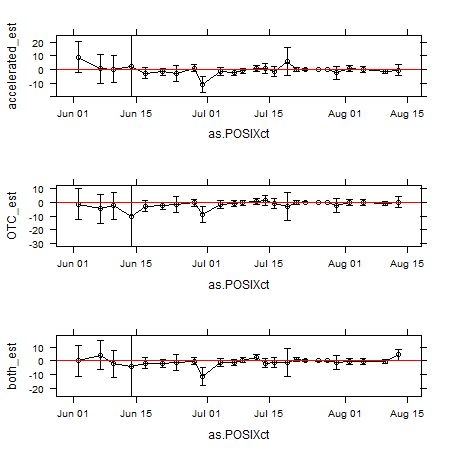
There is one more thorny issue that that author of the essay I linked above brings up and that’s the issue of what error rate to use for your confidence intervals. Do we need to Bonferroni correct them or otherwise adjust them? I would argue that we shouldn’t worry about this. As Rice (1989) points out, “there is no clear criterion for deciding when a simultaneous-inference test is required.” Rice suggests applying Bonferroni corrections when a group of two or more tests is scanned to see what is significant (i.e. a posteriori testing) or when two or more tests address a common null hypothesis. Sounds reasonable, but Cabin and Mitchell (2000) point out that it’s difficult to determine when either of these conditions are met. As my statistics handbook from my college stats class said, we may want to correct errors when we are trying to make statements such as “Some one or more of these are false.” I feel like I rarely need to make such an assertion and am thus not that bothered by the chance of having a higher groupwise error as long as I remember when inspecting the results that these are 95% and not 100% confidence intervals. For example, in the case of this data set, I don’t need to say “there is never a difference between our treatments.” Likewise, I can observe one date at which a “significant” difference is seen and disregard it as a fluke (e.g., the June 30 samples below where the controls were a little unusual).

Finally, here’s a graph of the results for the ammonium data, showing the mean differences±95%CI between each of our three treatments and the control. the three treatments are snowmelt acceleration, warming via open top chamber (OTC), and a both together. The overall conclusion here is that our treatments did not have a dramatic effect on ammonium at the times that we measured it, though we can be less sure about that conclusion at the beginning of the season.

xYplot(Cbind(accelerated_est,accelerated_lwr,accelerated_upr) ~
  as.POSIXct(strptime(ml.dun$date,"%Y-%m-%d")), type='b',
  data=ml.dun, panel=panel.xydiff)