HOT SPOTS PACKAGE TUTORIAL
This is a simple tutorial for using my R package hotspots that can be used to identify hot spots within spatial or temporal data sets. The hotspots package is designed to look within a set of measured values of a variable and identify values that are disproportionately high based on both the deviance of any given value from a statistical distribution and its similarity to other values. Because this relative magnitude of each value is taken into account, a value that is a statistical outlier may not always be a hot spot if other values are similarly large. There is a subjective cutoff for the deviance from the theoretical distribution, which is set by default to p = 0.99.
The main things you can do with the hot spot package are to calculate a hot spot cutoff (Ch) for your data set, plot a density plot (which is basically a "smoothed out histogram") of your data showing the hot spot cutoff and the hot spots, and calculate the magnitude of disproportionality for each value in the data set, where all hot spots have disproportionality > 1.
Here I'll show how most rapidly to get the package running and use it on your data. I will not delve into the math. After you get a feel for how it works, you can read the supplemental material in the paper [DOI] if you are curious about how the cutoff is calculated.
STEP 1. Install R: Windows Mac
STEP 2. Install the hotspots package. Open R, go to the packages menu, select "Install package(s)...", select a mirror that's close to you, then select the hotspots package and hit install. It will install a couple of dependent packages as well. If you need to choose where to look for the package, you want the "binary" package made for your OS (Windows or Mac). After it is installed, mount the package with:
library(hotspots)
STEP 3. Try out some of the functions on simulated data.
Example 1. Hot spot cutoff for randomly generated lognormally distributed data:
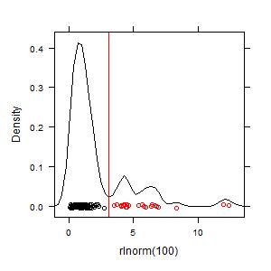
x <- rlnorm(100)
plot(hotspots(x))
Your graph should look something this:
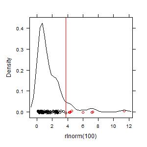
The key value that is calculated is the hot spot cutoff, Ch, which is shown as a red line in the graph. To see just that value:
hotspots(x)
To get more detailed information about the hot spot cutoff calculation and the importance of hot spots within the data set, do:
summary(hotspots(x))
The output:
Source data: rlnorm(100)
Distribution and probability: t, 0.99
Tail: positive hot spots only
Mean: 1.38764
Median: 0.89401
Min: 0.07207
Max: 7.66360
Qn: 0.76708
CV (Qn/median): 0.85803
n = 100
positive hot spots:
Cutoff number positive hot spots % positive hot spots % sum
3.679 7 7 26.5
Finally, calculate the disproportionality for each value (Hot spots have disproportionality > 1):
sort(disprop(hotspots(x))$positive)
Example 2. Greater skew in the data means more hot spots will be found:
plot(hotspots(rlnorm(100, sd = 2)))
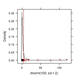
Their disproportionality will also be higher for the higher values
sort(disprop(hotspots(rlnorm(100, sd = 2)))$positive)
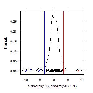
Example 3. Hot spots and reverse hot spots:
rln100pn <- hotspots(c(rlnorm(50),rlnorm(50)*-1),tail = "both")
summary(rln100pn)
plot(rln100pn)
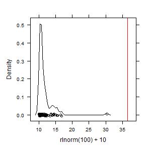
Example 4. For data that are skewed but all similarly large, no hot spots are found because values are not disproportionately large:
rln100p10 <- hotspots(rlnorm(100)+10)
summary(rln100p10)
plot(rln100p10)
Example 5. Changing the subjective parameter p to 0.90 instead of the default 0.99 will identify a greater number of hot spots:
plot(hotspots(rlnorm(100), p = 0.9))
More examples. Access the help files from within R:
?hotspots
?disprop
?plot.hotspots
?summary.hotspots
STEP 4. Try it on your own data. The guide for importing any kind of data into R is here in the "R Data Import/Export" manual. This step can be as simple as saving your spreadsheet as a .csv file and importing with a line of code. One basic tip is to make sure your .csv file is arranged one observation per row, one variable per column, preferably with simple column names that don't contain weird characters or spaces. Then import with something like this:
mydata <- read.csv("C:/Users/Anthony/Documents/mydata.csv", header = T)
Don't use forward slashes \ in files names. Once your data set is in R, you can see it by typing the object name (in the example above mydata) or see just the variable names by doing:
names(mydata)
If this simple import technique doesn't work, read the manual or talk to a friend who knows R. Once your data is in R, you can do any of the above analyses with any of the columns in your imported data. For example, if you have a variable called CO2:
plot(hotspots(mydata$CO2))
That's it. Please don't hesitate to contact me if you have questions:
anthony@darrouzet-nardi.net